Project for Patterns and Trends in Environmental Data - Computational Movement Analysis
Author
Mirjam Scheib & Miriam Steinhauer
Published
July 2, 2023
1 BACKGROUND AND RESEARCH QUESTIONS
It is known that several factors like the weather condition (Brum-Bastos et al., 2018; Guo et al., 2022), the day of the week and time of the day (Liu et al., 2020; Sathishkumar et al., 2020) influence spatio-temporal movement patterns of people. There are several studies investigating movement patterns of people in urban areas with the aim to improve the distribution of facilities and the provisioning of transportation services, as well as to manage traffic peaks (Kyaing et al., 2017; Liu et al., 2020). It was shown that travel behaviour is significantly impacted by age, income and life stage influencing travelling behaviour in different ways (Kattiyapornpong & Miller, 2009). Because people with different socio-demographic variables follow distinct spatio-temporal movement patterns, we investigate the travelling behaviour of 11 students in this project work. The canton of Zurich accommodates the most students in Switzerland, with numbers continuing to rise (Bundesamt für Statistik, 2023; Medienmitteilung Kanton ZH, 2021). Additionally, students and apprentices (from the age of 15 years) make up 39 % of the public transport commuter mass, which is why detailed knowledge of spatio-temporal patterns of students could help to manage public transport infrastructure (Bundesamt für Statistik, 2021). Therefore, we want to investigate the influence of three environmental factors on spatio-temporal movement patterns of students, aiming to answer the following research questions:
Does the day of the week (weekend vs. weekday) have an influence on the spatio-temporal movement patterns of students?
Does the time of the day compared between weekend and weekday have an influence on the spatio-temporal movement patterns of students?
Does intense precipitation have an impact on spatio-temporal movement patterns of students?
2 DATA & METHODS
2.1 Data
Primary data used in this project work consisted of trajectory data from 11 students collected with the Posmo App containing the following attributes:
user_id: entails the individual ID of the user (= student) (type: character)
datetime: date and time when a position of a user is tracked (type: datetime)
weekday: abbreviated name of the weekday (e.g. Mon = Monday) (type: character)
place_name: names of a place, in which a user is at a specific time (type: character)
transport_mode: the type of transport used by a user (e.g. car, bicycle, foot, train, other….) (type: character)
lon_x/lat_y: coordinates of the user at a specific time (type: numeric)
Additionally, precipitation data consisting of measurement every 10 minutes from 84 stations in the canton of Zurich and bordering cantons (SZ, AG, ZG, TG, SG) was used to investigate the influence of precipitation on spatio-temporal movement patterns of students.
2.2 Pre-processing
First we reviewed data consistency by creating a point plot, where every tracking point in time (x-axis) was displayed per user (y-axis). Five students needed to be eliminated due to insufficient tracking point coverage in time (Fig. 1). Additionally, the dataset was cut into a specific timeframe (28.04.2023 - 09.05.2023) covering 11 days to ensure sufficient overlap of tracking points between users (Fig. 2).
Figure 1: Point plot of every tracking point in time (x-axis) displayed per student (y-axis). Posmo4, posmo7, posmo8, posmo9 and posmo 10 needed to be eliminated due to insufficient tracking point coverage in time.
Figure 2: Point plot of every tracking point in time (x-axis) displayed per student (y-axis). The dataset consisting of 6 students was cut into a timespan covering 11 days to ensure sufficient tracking point coverage for every student.
Additionally, travel modes consisting of “Airplane”, “Funicular” and “Other1” were removed, as they presented either too specific or unspecific travel modes to be of interest in the subsequent analysis. Furthermore, the annotation of all convenience variables are considered crucial pre-processing steps for the subsequent analysis. First, it was discriminated between weekend (Sa – So) and weekdays (Mo – Fr). Additionally, to discriminate between days with high and low/no precipitation we calculated the nearest weather station for every trajectory point and annotated the precipitation data at the matching time to our dataset. For this we created a new column in the posmo dataset, to create a time join key matching the 10 minutes interval of the weather data. We considered a precipitation of > 20 mm per 24 hours as a day with intense precipitation, as MeteoSwiss (2023) defines a precipitation from 10 – 30 mm per 24 hours as high intensity precipitation.
To investigate spatio-temporal movement patterns of students in concern to environmental variables, we discriminated between static and movement segments and assigned to every moving sequence a segment ID. From this we calculated distance, speed and duration for every segment.
All pre-processing steps can be accessed in a separate quarto-file (Pre_Processing.qmd) in our github respiratory under the following link: https://github.com/mirjamscheib/Semester_Project.git
2.3 Analysis
The analysis of the research questions was carried out by creating summary tables and boxplots to investigate distance, speed and duration of different travel modes comparing weekends with weekdays and high precipitation with no precipitation. Additionally, line plots visualizing distance, speed and duration per hour of the day comparing weekends with weekdays were carried out. Cartographic maps visualizing trajectory points of students comparing weekends with weekdays and precipitation and no precipitation complement the analysis.
Code
# clear space rm(list=ls())# load packages library("readr")library("dplyr")library("ggplot2")library("sf")library("terra")library("tmap")library("gitcreds")library("dplyr")library("SimilarityMeasures")library("lubridate")library("plotly")# load clean data posmo <-read_delim("posmo_data/posmo_trips.csv")
3 RESULTS
3.1 Impact of the day of the week
3.1.1 Spatial Analysis
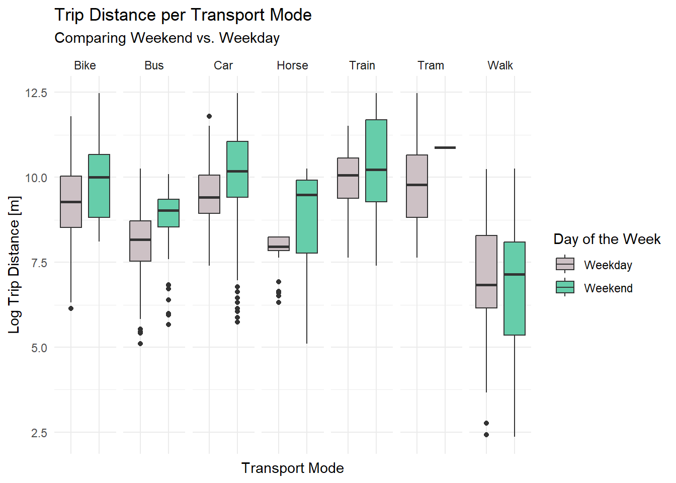
A higher trip distance resulted for every travel mode on weekends compared to weekdays. Generally, the distance travelled by foot (travel mode: walk) had a lower mean than other travel modes. On the contrary it can be seen, that the mean distance travelled by bike is in the same range as the travel modes car and train.
Code
ggplot() +geom_boxplot(data = posmo, aes(day_week, log(trip_dis), fill = day_week)) +labs(title ="Trip Distance per Transport Mode", subtitle ="Comparing Weekend vs. Weekday", fill ="Day of the Week") +ylab("Log Trip Distance [m]") +xlab("Transport Mode") +scale_fill_manual(values =c("weekday"="lavenderblush3", "weekend"="aquamarine3"), labels =c( "Weekday", "Weekend")) +facet_wrap(~transport_mode, nrow =1) +theme_minimal() +theme(axis.text.x=element_blank())
Figure 3: Trip distance per transport mode compared between weekends and weekdays, the trip distance is logarythmised
There is a tendency of trip speed being higher on the weekends than during the week except for the travel mode train, where the relationship is reversed. Again, we find the mean trip speed by bike being in a similar range as when students travelled by car and train, whereas the travel mode bus conforms to when students travelled by horse.
Code
ggplot(posmo, aes(day_week, log(trip_speed), fill = day_week)) +geom_boxplot() +labs(title ="Trip Speed per Transport Mode", subtitle ="Comparing Weekend vs. Weekday", fill ="Day of the Week") +ylab("Log Speed [m/s]") +xlab("Transport Mode") +scale_fill_manual(values =c("weekday"="lavenderblush3", "weekend"="aquamarine3"), labels =c( "Weekday", "Weekend")) +facet_wrap(~transport_mode, nrow =1) +theme_minimal() +theme(axis.text.x=element_blank())
Figure 4: Trip speed per transport mode compared between weekends and weekdays, the trip speed is logarythmised
3.1.2 Temporal Analysis
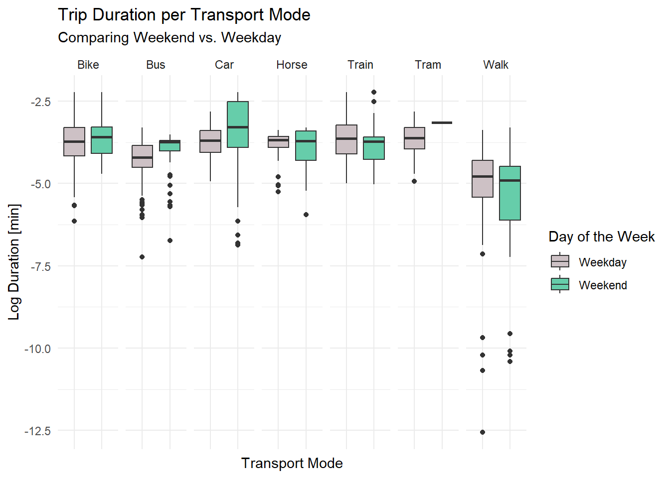
The trip duration shows no clear trend, as the results appear heterogeneous between weekends and weekdays for every travel mode considered. There is however a tendency, that the mean trip duration is lower when students are travelling by foot compared to all other travel modes.
Code
#| label: Boxplot comparing trip duration between weekend and weekday of travelmodesggplot() +geom_boxplot(data = posmo, aes(day_week, log(trip_duration/60), fill = day_week)) +labs(title ="Trip Duration per Transport Mode", subtitle ="Comparing Weekend vs. Weekday", fill ="Day of the Week") +ylab("Log Duration [min]") +xlab("Transport Mode") +scale_fill_manual(values =c("weekday"="lavenderblush3", "weekend"="aquamarine3"), labels =c( "Weekday", "Weekend")) +facet_wrap(~transport_mode, nrow =1) +theme_minimal() +theme(axis.text.x=element_blank())
Figure 5: Trip duration per transport mode compared between weekends and weekdays, the trip duration is logarythmised
3.1.3 Cartographic Representation
Code
# transform posmo data into an sf object posmo <-st_as_sf(posmo, coords =c("X","Y"), crs =2056) # 1. add grouping variable to the sf objectposmo_grouped <-group_by(posmo, dataset)# 2. use summarise() to "dissolve" all point into a multipoint objectposmo_smry <-summarise(posmo_grouped)# 3. run st_convex_hull()mcp_posmo <-st_convex_hull(posmo_smry)# set visual modetmap_mode("view")# cartographic visualisation tm_shape(mcp_posmo) +tm_fill(col ="dataset", alpha =0.4, title ="Student") +tm_shape(mcp_posmo) +tm_borders(col ="black") +tm_shape(posmo) +tm_dots(col ="day_week", title ="Day of the Week")
Figure 6: Cartographic representation of trajectory points from six students compared between weekends and weekdays
3.2 Impact of the time of the day
Code
# load clean data posmo <-read_delim("posmo_data/posmo_trips.csv")# round datetime to 1h posmo_round <- posmo |>mutate(hour = lubridate::hour(datetime))# create dataframe, which calculates mean steplength, speed per hour over all dates comparing weekends and weekdaysposmo_day <- posmo_round |>group_by(hour, day_week)|>summarise(mean_dis =mean(trip_dis, na.rm =TRUE),mean_speed =mean(trip_speed, na.rm =TRUE),mean_duration =mean(trip_duration, na.rm =TRUE))
3.2.1 Spatial Analysis
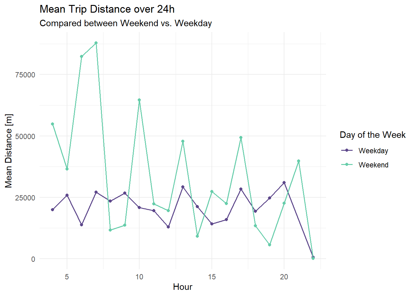
The trip distance per hour shows a higher trip distance on the weekends compared to weekdays. After a peak of travelled distance at around 7 AM on the weekend, a decreasing trend of distance per hour is shown, with regular peaks (10 AM, 1 PM, 5 PM, 9 PM). The trip distance per hour during the week shows a rather balanced pattern with regular peaks during the day (5 AM, 7 AM, 9 AM, 1 PM, 5 PM, 8 PM) with the highest peaks at around 1 PM, 5 PM and 8 PM.
Code
#| label: Mean trip distance per hour of the day compared between weekend/weekdayggplot(posmo_day, aes(hour, mean_dis, col = day_week)) +geom_point() +geom_line(lwd =0.7) +labs(title ="Mean Trip Distance over 24h", subtitle ="Compared between Weekend vs. Weekday", color ="Day of the Week") +scale_color_manual(values =c("weekday"="mediumpurple4", "weekend"="aquamarine3"), labels =c("Weekday", "Weekend")) +ylab("Mean Distance [m]") +xlab("Hour") +theme_minimal()
Figure 7: Mean trip distance for every hour of the day compared between weekdays and weekends
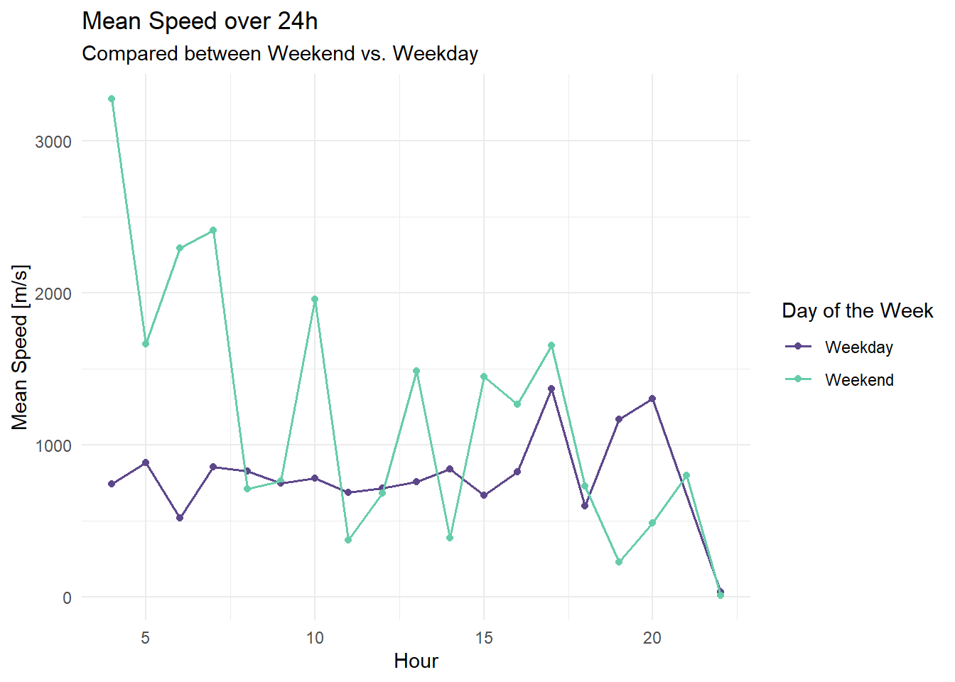
The trip speed shows a decreasing trend from around 4 AM to 11 PM on the weekend. Additionally, trip speed per hour is mostly higher for weekends compared to weekdays. On weekdays the trip speed per hour is relatively stable during the day (7 AM to 4 PM) with two peaks at around 5 PM and 8 PM and a considerably lower speed at around 6 AM.
Code
ggplot(posmo_day, aes(hour, mean_speed, col = day_week)) +geom_point() +geom_line(lwd =0.7) +labs(title ="Mean Speed over 24h", subtitle ="Compared between Weekend vs. Weekday", color ="Day of the Week") +scale_color_manual(values =c("weekday"="mediumpurple4", "weekend"="aquamarine3"), labels =c("Weekday", "Weekend"))+ylab("Mean Speed [m/s]") +xlab("Hour") +theme_minimal()
Figure 8: Mean trip speed for every hour of the day compared between weekdays and weekends
3.2.2 Temporal Analysis
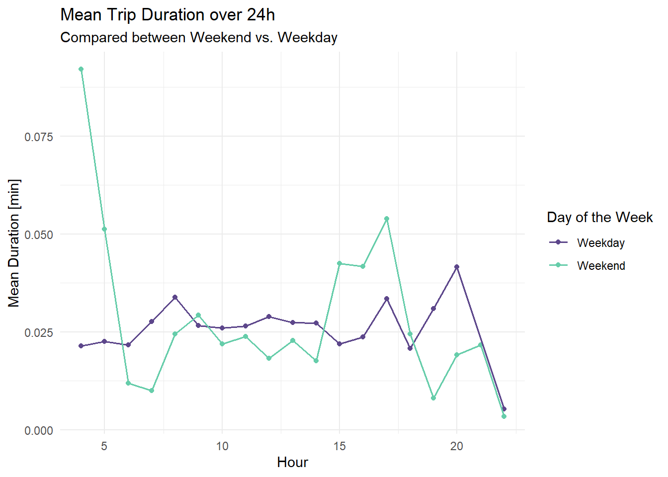
The trip duration reaches its peak at around 4 AM on the weekends, while on the weekdays the peak is at around 8 PM. Additionally, between 3 and 5 PM trip duration is considerably higher than the average on the weekend, where during the week the trip duration is higher at around 8 AM and 5 PM compared to other hours of the day.
Code
ggplot(posmo_day, aes(hour, mean_duration/60, col = day_week)) +geom_point() +geom_line(lwd =0.7) +labs(title ="Mean Trip Duration over 24h", subtitle ="Compared between Weekend vs. Weekday", color ="Day of the Week") +ylab("Mean Duration [min]") +xlab("Hour") +scale_color_manual(values =c("weekday"="mediumpurple4", "weekend"="aquamarine3"), labels =c("Weekday", "Weekend")) +theme_minimal()
Figure 9: Mean trip duration for every hour of the day compared between weekdays and weekends
3.3 Impact of precipitation
3.3.1 Spatial Analysis
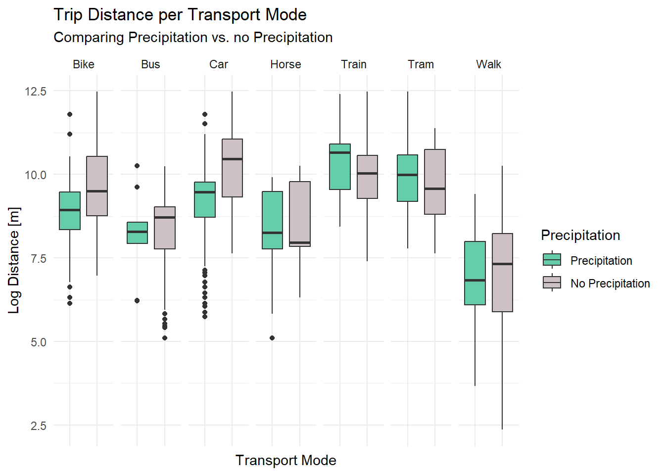
Precipitation reduced trip distance by bike, foot, bus and car, while the trip distance was higher for travel modes like train and tram. Rain does not seem to have an effect on trip distance when travelling by horse. Although, travel distances are impacted by precipitation, the effect can be described as heterogeneous.
Code
#| label: mean trip distance depending on precipitationggplot() +geom_boxplot(data = posmo, aes(rain_day, log(trip_dis), fill = rain_day)) +labs(title ="Trip Distance per Transport Mode", subtitle ="Comparing Precipitation vs. no Precipitation", fill ="Precipitation") +ylab("Log Distance [m]") +xlab("Transport Mode") +scale_fill_manual(values =c("rain"="lavenderblush3", "no_rain"="aquamarine3"), labels =c( "Precipitation", "No Precipitation")) +facet_wrap(~transport_mode, nrow =1) +theme_minimal() +theme(axis.text.x=element_blank())
Figure 10: Mean trip distance compared between precipiation and no/low precipitaion, where the trip distance is logarythmised
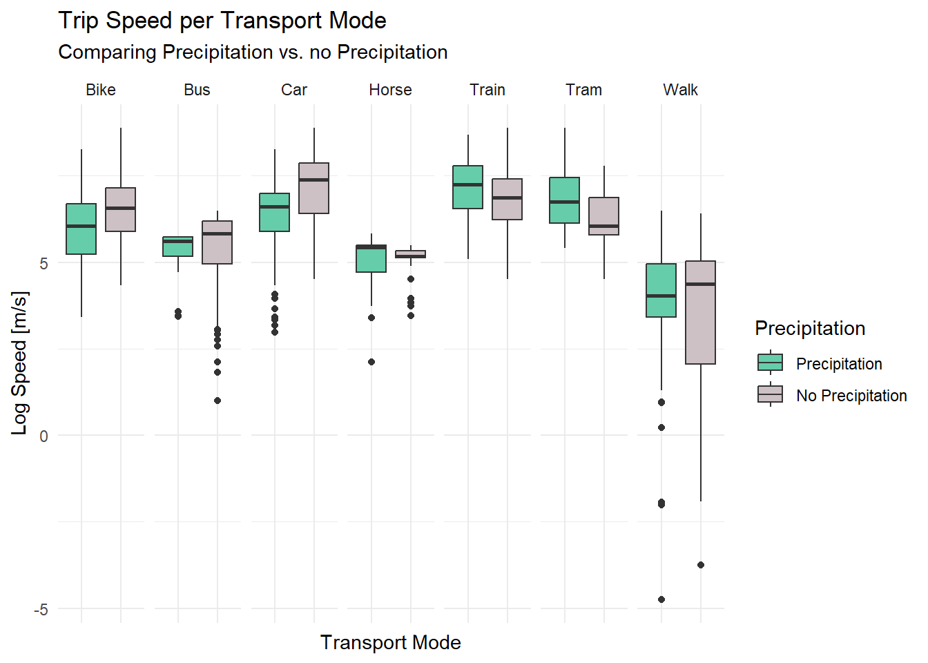
Trip speed at high precipitation is lower when travelling by bike, foot, bus and car, while for travel modes such as train and tram speed was higher. Travelling by horse does not seem to be effected by precipitation. Although, travel speeds are impacted by precipitation, the effect can be described as heterogeneous.
Code
ggplot(posmo, aes(rain_day, log(trip_speed), fill = rain_day)) +geom_boxplot() +labs(title ="Trip Speed per Transport Mode", subtitle ="Comparing Precipitation vs. no Precipitation", fill ="Precipitation") +ylab("Log Speed [m/s]") +xlab("Transport Mode") +scale_fill_manual(values =c("rain"="lavenderblush3", "no_rain"="aquamarine3"), labels =c( "Precipitation", "No Precipitation")) +facet_wrap(~transport_mode, nrow =1) +theme_minimal() +theme(axis.text.x=element_blank())
Figure 11: Mean trip speed compared between precipiation and no/low precipitaion, where the trip speed is logarythmised
3.3.2 Temporal Analysis
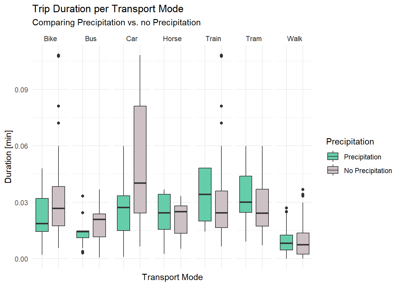
The duration of trips was shorter under heavy precipitation by bike, bus and car, while students travelled longer by train and tram. Considering travelling by horse and foot, precipitation does not seem to have an effect on trip duration.
Code
ggplot() +geom_boxplot(data = posmo, aes(rain_day, trip_duration/60, fill = rain_day)) +labs(title ="Trip Duration per Transport Mode", subtitle ="Comparing Precipitation vs. no Precipitation", fill ="Precipitation") +ylab("Duration [min]") +xlab("Transport Mode") +scale_fill_manual(values =c("rain"="lavenderblush3", "no_rain"="aquamarine3"), labels =c( "Precipitation", "No Precipitation")) +facet_wrap(~transport_mode, nrow =1) +theme_minimal() +theme(axis.text.x=element_blank())
Figure 12: Mean trip duration compared between precipiation and no/low precipitaion
3.3.3 Cartographic Representation
Code
# load weather stations legend <-read_delim("data/weather_legend.csv")# create sf object of joined dataweather <-st_as_sf(legend, coords =c("E","N"), crs =2056)# transform posmo data into an sf object posmo <-st_as_sf(posmo, coords =c("X","Y"), crs =2056) # 1. add grouping variable to the sf objectposmo_grouped <-group_by(posmo, dataset)# 2. use summarise() to "dissolve" all point into a multipoint objectposmo_smry <-summarise(posmo_grouped)# 3. run st_convex_hull()mcp_posmo <-st_convex_hull(posmo_smry)#choose map modetmap_mode("view")# segmented visualisation tm_shape(mcp_posmo) +tm_fill(col ="dataset", alpha =0.4, title ="Student") +tm_shape(mcp_posmo) +tm_borders(col ="black") +tm_shape(posmo) +tm_dots(col ="rain_day", title ="Precipitation") +tm_shape(weather) +tm_dots(title ="weather Stations")
Figure 13: Cartographic representation of trajectory points from six students compared between precipitation and no/low precipitation. Additionally, all weather stations used are visualised as black points on the map.
4 DISCUSSION
It is to be noted, that the investigated spatio-temporal movement patterns of students cannot be generalized for the general population, as it was shown that sociodemographics and travel behaviour of university students differ from the general population, as well as between students living on or off campus and students attending urban or suburban campuses (Khattak et al., 2011). Furthermore, conclusions that can be drawn by investigating our three environmental factor individually are limited, as these factors interact with each other and several additional factors lead to differences of time expenditure on different travel modes such as for example temperature and gender. Multi-channel sequence analysis (MCSA) are therefore particularly relevant to study human mobility as they are able to simultaneously consider multiple environmental variables (Brum-Bastos et al., 2018).
Additionally, during the course of this project it became clear, that the Posmo App comes with severe uncertainties and tracking errors. Quantifying those uncertainties would be subject to another semester project in itself, which is why we assumed that the data we used was correct and interpreted it as such.
4.1 Patterns of the day of the week
The day of the week impacted spatio-temporal movement patterns of students, where movement activity regarding trip distance and speed was generally slightly higher on the weekends than during the week.
Looking at the use of bikes Sathishkumar et al. (2020) found, that most bike trips during the week took around 24 minutes compared to 30 minutes on the weekends, which aligns with our results, where bike trip duration was slightly higher on weekends. Additionally, the use of public transport during weekdays are only slightly higher in distance, speed and sometimes lower in duration, which could indicate, that other factors than only the weekday impact the spatio-temporal movement of students over different travel modes. In line with this Brum-Bastos et al. (2018) found, that rain has no key role on travel modes during the weekend, but heavy rain decreases the use of public transport during the week. Precipitation was a factor influencing 8 of 11 investigated days.
Since trip distance, duration and speed are interconnected parameters and the pattern is clear for trip distance and gets weaker for speed and becomes unrecognizable for trip duration, a reason could be our imbalanced dataset. As we had to cut our datasets in time, to attain seamless data over all days, from all individual participants, we ended up with seven days of the data for weekdays and only four days for weekends. This bias potentially has impacted our results. For further studies we therefore suggest a larger number of participants and a longer period of GPS-tracking, to achieve a more balanced dataset.
4.2 Patterns of the time of the day
The time of the day impacted spatio-temporal movement patterns of students compared between weekend and weekdays, where generally higher movement activity per hour could be observed during weekends. Spatio-temporal movement during the week was more balanced, with lower peaks of distance, speed and duration during the day. In contrast, high peaks of trip distance, speed and duration were found on the weekends, early in the morning, with a general trend to decrease during the day, often times with regular peaks.
Comparing our results to literature, the movement pattern Sathishkumar et al. (2020) found, considering only the travel mode bike, stays in contrast to our results found for the weekend, where there is the shortest trip duration around 8 AM and the trips are the longest in the afternoon and evening. However, in their study there was no distinction between weekend and weekday, as well as only one travel mode was investigated, making the comparison to our results difficult. Ryan et al. (2010) and Brum-Bastos et al. (2018) found more varied activities on weekends, which aligns with our findings of generally more peaks and higher movement activity during the day on the weekends, which they explain by having more scope for freedom of action on weekends compared to external controls during the week. When looking at movement activity during the day, it was shown that daylight impact movement behaviour of humans, where less daylight results in less time walking, time spend on public transport and more vehicular use during the weekdays. On weekends this trend reverses, where walking and public transport become more prominent during night hours, while vehicle use is more prominent during daylight hours (Brum-Bastos et al., 2018). Additionally, more time at home and less time shopping or socializing is spent during night hours during the week while again, this relationship reverses on the weekends (Brum-Bastos et al., 2018). This fits with our observations, as we found a high peak of movement activity during 3 to 6 AM on the weekends, as well as more and higher peaks of movement activity on the weekends. During the weekdays the patterns of distance, speed and duration were found to be more homogeneous with lower peaks, fitting our expectation of an increase in activity of spatio-temporal movement behaviour during commuting times (around 6 – 8 AM and 3 – 6 PM) . An additional peak for distance, speed and duration at around 8 PM during the weekdays could be explained by leisure activities in the evening.
4.3 Precipiation Patterns
Precipitation impacted spatio-temporal movement patterns of students in a hetergoeneous way, indicating no clear relationship between precipitation and movement activity in general. However, some patterns were emerging as the movement (distance, speed, and duration) of students was reduced under heavy rain when travelling by bike, bus and car, while it was increased when travelling by train and tram. These results are in contrast to Brum-Bastos et al. (2018), where they found a general trend of more vehicular use under heavy rain, while in our study we found a general decrease in the use of cars.
It could be shown that speed and distance were lower under heavy rain when travelling by foot, while the duration was not impacted by precipitation patterns. In contrast to our finding, Brum-Bastos et al. (2018) found an overall decrease in walking during rain. It was shown, that when travel destinations are obligatory (e.g., work, lectures) people change their travel mode more likely under heavy rain, meaning that they drive to work instead of walk. However, if destinations are linked to leisure activities, people more likely just postpone the task instead of changing their travel mode (Connolly, 2008). Additionally, during the week a decrease in public transport was observed under heavy rain by Brum-Bastos et al. (2018). This finding are in contrast to our results, where the use of some public transport means (train and tram) was increased under heavy rain, although we did not include the consideration of the days of the week.
However, it is to be said that those patterns found in our data are not indicative, as we only had a sample size of 6 students and investigated 11 days, from which 8 days were considered having heavy rainfall. Additionally, the results need to be interpreted with caution, as for some trajectory points the weather stations are rather far away to serve as an indication for precipitation (figure 13).
5 SOURCES
5.1 Data
Trajectory data of students: Posmo App
Weather data: https://gate.meteoswiss.ch/idaweb
5.2 Literature
Brum-Bastos, V. S., Long, J. A., & Demšar, U. (2018). Weather effects on human mobility: A study using multi-channel sequence analysis. Computers, Environment and Urban Systems, 71, 131–152. https://doi.org/10.1016/j.compenvurbsys.2018.05.004
Bundesamt für Statistik. (2021). Pendlermobilität. Bundesamt für Statistik. https://www.bfs.admin.ch/bfs/de/home/statistiken/mobilitaet-verkehr/personenverkehr/pendlermobilitaet.html
Bundesamt für Statistik. (2023, March 28). Studierende an den universitären Hochschulen: Basistabellen - 1990-2022 | Tabelle. Bundesamt für Statistik. https://www.bfs.admin.ch/asset/de/24345359
Connolly, M. (2008). Here Comes the Rain Again: Weather and the Intertemporal Substitution of Leisure. Source Journal of Labor Economics Journal of Labor Economics, 26(1), 73–100. https://doi.org/10.1086/522067
Guo, P., Sun, Y., Chen, Q., Li, J., & Liu, Z. (2022). The Impact of Rainfall on Urban Human Mobility from Taxi GPS Data. Sustainability, 14(15), Article 15. https://doi.org/10.3390/su14159355
Kattiyapornpong, U., & Miller, K. E. (2009). Socio‐demographic constraints to travel behavior. International Journal of Culture, Tourism and Hospitality Research, 3(1), 81–94. https://doi.org/10.1108/17506180910940360
Khattak, A., Wang, X., Son, S., & Agnello, P. (2011). Travel by University Students in Virginia: Is This Travel Different from Travel by the General Population? Transportation Research Record: Journal of the Transportation Research Board, 2255(1). https://doi.org/10.3141/2255-15
Kyaing, K., Lwin, K., & Sekimoto, Y. (2017). Human mobility patterns for different regions in Myanmar based on CDRs data. IPTEK Journal of Proceedings Series, 3(6).
Liu, X., Sun, L., Sun, Q., & Gao, G. (2020). Spatial Variation of Taxi Demand Using GPS Trajectories and POI Data. Journal of Advanced Transportation, 2020, e7621576. https://doi.org/10.1155/2020/7621576
Medienmitteilung Kanton ZH. (2021). Bildung in Zahlen. Kanton Zürich. https://www.zh.ch/de/news-uebersicht/medienmitteilungen/2021/07/bildung-in-zahlen.html
MeteoSwiss. (2023). Precipitation. Federal Office of Meterology and Climatology MeteoSwiss. Retrieved 19 June 2023, from https://www.meteoschweiz.admin.ch/wetter/wetter-und-klima-von-a-bis-z/niederschlag.html
Ryan, R. M., Bernstein, J. H., & Brown, K. W. (2010). Weekends, Work, and Well-Being: Psychological Need Satisfactions and Day of the Week Effects on Mood, Vitality, and Physical Symptoms. Journal of Social and Clinical Psychology, 29(1), 95–122. https://doi.org/10.1521/jscp.2010.29.1.95
Sathishkumar, Cho, Y., & Jangwoo, Park. (2020). Seoul bike trip duration prediction using data mining techniques. IET Intelligent Transport Systems, 14(11), 1465–1474. https://doi.org/10.1049/iet-its.2019.0796
Source Code
---title: "Effects of three environmental factors on spatio-temporal movement patterns of students"subtitle: "Project for Patterns and Trends in Environmental Data - Computational Movement Analysis"author: "Mirjam Scheib & Miriam Steinhauer"date: "07/02/2023"format: html: code-fold: true code-tools: true code-line-numbers: truehighlight-style: pygmentstable-of-contents: truenumber-sections: trueexecute: echo: true message: false eval: true warning: falseeditor: markdown: wrap: 72---# BACKGROUND AND RESEARCH QUESTIONSIt is known that several factors like the weather condition (Brum-Bastoset al., 2018; Guo et al., 2022), the day of the week and time of the day(Liu et al., 2020; Sathishkumar et al., 2020) influence spatio-temporalmovement patterns of people. There are several studies investigatingmovement patterns of people in urban areas with the aim to improve thedistribution of facilities and the provisioning of transportationservices, as well as to manage traffic peaks (Kyaing et al., 2017; Liuet al., 2020). It was shown that travel behaviour is significantlyimpacted by age, income and life stage influencing travelling behaviourin different ways (Kattiyapornpong & Miller, 2009). Because people withdifferent socio-demographic variables follow distinct spatio-temporalmovement patterns, we investigate the travelling behaviour of 11students in this project work. The canton of Zurich accommodates themost students in Switzerland, with numbers continuing to rise (Bundesamtfür Statistik, 2023; Medienmitteilung Kanton ZH, 2021). Additionally,students and apprentices (from the age of 15 years) make up 39 % of thepublic transport commuter mass, which is why detailed knowledge ofspatio-temporal patterns of students could help to manage publictransport infrastructure (Bundesamt für Statistik, 2021). Therefore, wewant to investigate the influence of three environmental factors onspatio-temporal movement patterns of students, aiming to answer thefollowing research questions:1. Does the day of the week (weekend vs. weekday) have an influence on the spatio-temporal movement patterns of students?2. Does the time of the day compared between weekend and weekday have an influence on the spatio-temporal movement patterns of students?3. Does intense precipitation have an impact on spatio-temporal movement patterns of students?# DATA & METHODS## DataPrimary data used in this project work consisted of trajectory data from11 students collected with the Posmo App containing the followingattributes:- **user_id:** entails the individual ID of the user (= student) (type: character)- **datetime:** date and time when a position of a user is tracked (type: datetime)- **weekday:** abbreviated name of the weekday (e.g. Mon = Monday) (type: character)- **place_name:** names of a place, in which a user is at a specific time (type: character)- **transport_mode:** the type of transport used by a user (e.g. car, bicycle, foot, train, other....) (type: character)- **lon_x/lat_y:** coordinates of the user at a specific time (type: numeric)Additionally, precipitation data consisting of measurement every 10minutes from 84 stations in the canton of Zurich and bordering cantons(SZ, AG, ZG, TG, SG) was used to investigate the influence ofprecipitation on spatio-temporal movement patterns of students.## Pre-processingFirst we reviewed data consistency by creating a point plot, where everytracking point in time (x-axis) was displayed per user (y-axis). Fivestudents needed to be eliminated due to insufficient tracking pointcoverage in time (Fig. 1). Additionally, the dataset was cut into aspecific timeframe (28.04.2023 - 09.05.2023) covering 11 days to ensuresufficient overlap of tracking points between users (Fig. 2).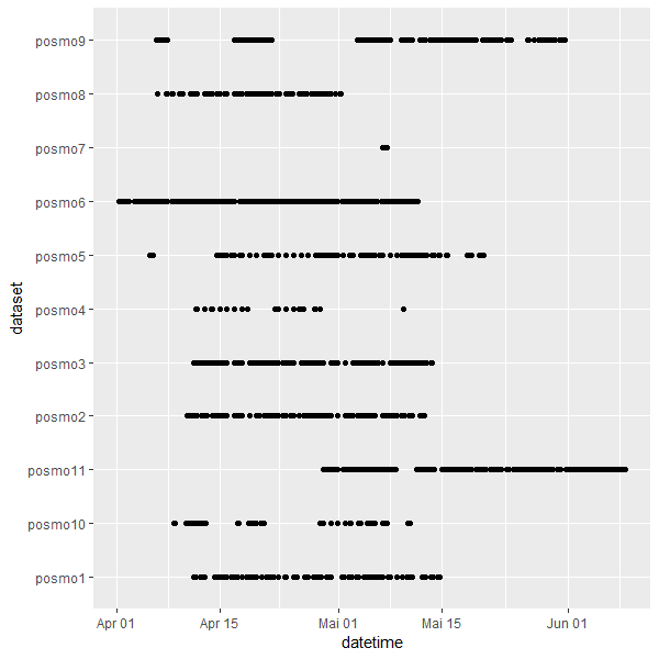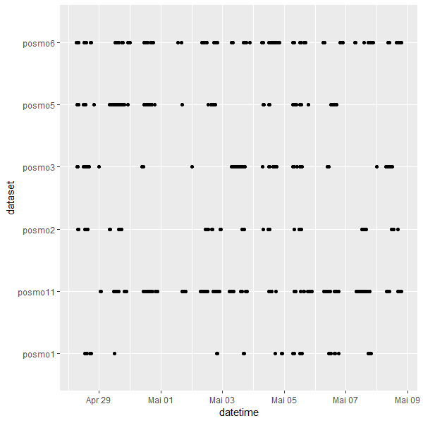Additionally, travel modes consisting of "Airplane", "Funicular" and"Other1" were removed, as they presented either too specific orunspecific travel modes to be of interest in the subsequent analysis.Furthermore, the annotation of all convenience variables are consideredcrucial pre-processing steps for the subsequent analysis. First, it wasdiscriminated between weekend (Sa -- So) and weekdays (Mo -- Fr).Additionally, to discriminate between days with high and low/noprecipitation we calculated the nearest weather station for everytrajectory point and annotated the precipitation data at the matchingtime to our dataset. For this we created a new column in the posmodataset, to create a time join key matching the 10 minutes interval ofthe weather data. We considered a precipitation of \> 20 mm per 24 hoursas a day with intense precipitation, as MeteoSwiss (2023) defines aprecipitation from 10 -- 30 mm per 24 hours as high intensityprecipitation.To investigate spatio-temporal movement patterns of students in concernto environmental variables, we discriminated between static and movementsegments and assigned to every moving sequence a segment ID. From thiswe calculated distance, speed and duration for every segment.All pre-processing steps can be accessed in a separate quarto-file(Pre_Processing.qmd) in our github respiratory under the following link:https://github.com/mirjamscheib/Semester_Project.git## AnalysisThe analysis of the research questions was carried out by creatingsummary tables and boxplots to investigate distance, speed and durationof different travel modes comparing weekends with weekdays and highprecipitation with no precipitation. Additionally, line plotsvisualizing distance, speed and duration per hour of the day comparingweekends with weekdays were carried out. Cartographic maps visualizingtrajectory points of students comparing weekends with weekdays andprecipitation and no precipitation complement the analysis.```{r}#| label: load packages and clean data# clear space rm(list=ls())# load packages library("readr")library("dplyr")library("ggplot2")library("sf")library("terra")library("tmap")library("gitcreds")library("dplyr")library("SimilarityMeasures")library("lubridate")library("plotly")# load clean data posmo <-read_delim("posmo_data/posmo_trips.csv")```# RESULTS## Impact of the day of the week### Spatial AnalysisA higher trip distance resulted for every travel mode on weekendscompared to weekdays. Generally, the distance travelled by foot (travelmode: walk) had a lower mean than other travel modes. On the contrary itcan be seen, that the mean distance travelled by bike is in the samerange as the travel modes car and train.```{r, fig.cap = "Figure 3: Trip distance per transport mode compared between weekends and weekdays, the trip distance is logarythmised"}#| label: Boxplot comparing trip distance between weekend and weekday of travelmodesggplot() +geom_boxplot(data = posmo, aes(day_week, log(trip_dis), fill = day_week)) +labs(title ="Trip Distance per Transport Mode", subtitle ="Comparing Weekend vs. Weekday", fill ="Day of the Week") +ylab("Log Trip Distance [m]") +xlab("Transport Mode") +scale_fill_manual(values =c("weekday"="lavenderblush3", "weekend"="aquamarine3"), labels =c( "Weekday", "Weekend")) +facet_wrap(~transport_mode, nrow =1) +theme_minimal() +theme(axis.text.x=element_blank())```There is a tendency of trip speed being higher on the weekends thanduring the week except for the travel mode train, where the relationshipis reversed. Again, we find the mean trip speed by bike being in asimilar range as when students travelled by car and train, whereas thetravel mode bus conforms to when students travelled by horse.```{r, fig.cap = "Figure 4: Trip speed per transport mode compared between weekends and weekdays, the trip speed is logarythmised"}#| label: Boxplot comparing trip speed between weekend and weekday of travelmodesggplot(posmo, aes(day_week, log(trip_speed), fill = day_week)) +geom_boxplot() +labs(title ="Trip Speed per Transport Mode", subtitle ="Comparing Weekend vs. Weekday", fill ="Day of the Week") +ylab("Log Speed [m/s]") +xlab("Transport Mode") +scale_fill_manual(values =c("weekday"="lavenderblush3", "weekend"="aquamarine3"), labels =c( "Weekday", "Weekend")) +facet_wrap(~transport_mode, nrow =1) +theme_minimal() +theme(axis.text.x=element_blank())```### Temporal AnalysisThe trip duration shows no clear trend, as the results appearheterogeneous between weekends and weekdays for every travel modeconsidered. There is however a tendency, that the mean trip duration islower when students are travelling by foot compared to all other travelmodes.```{r, fig.cap = "Figure 5: Trip duration per transport mode compared between weekends and weekdays, the trip duration is logarythmised"}#| label: Boxplot comparing trip duration between weekend and weekday of travelmodesggplot() +geom_boxplot(data = posmo, aes(day_week, log(trip_duration/60), fill = day_week)) +labs(title ="Trip Duration per Transport Mode", subtitle ="Comparing Weekend vs. Weekday", fill ="Day of the Week") +ylab("Log Duration [min]") +xlab("Transport Mode") +scale_fill_manual(values =c("weekday"="lavenderblush3", "weekend"="aquamarine3"), labels =c( "Weekday", "Weekend")) +facet_wrap(~transport_mode, nrow =1) +theme_minimal() +theme(axis.text.x=element_blank())```### Cartographic Representation```{r, fig.cap = "Figure 6: Cartographic representation of trajectory points from six students compared between weekends and weekdays"}#| label: prepro and creation of visual map with convex hull# transform posmo data into an sf object posmo <-st_as_sf(posmo, coords =c("X","Y"), crs =2056) # 1. add grouping variable to the sf objectposmo_grouped <-group_by(posmo, dataset)# 2. use summarise() to "dissolve" all point into a multipoint objectposmo_smry <-summarise(posmo_grouped)# 3. run st_convex_hull()mcp_posmo <-st_convex_hull(posmo_smry)# set visual modetmap_mode("view")# cartographic visualisation tm_shape(mcp_posmo) +tm_fill(col ="dataset", alpha =0.4, title ="Student") +tm_shape(mcp_posmo) +tm_borders(col ="black") +tm_shape(posmo) +tm_dots(col ="day_week", title ="Day of the Week")```## Impact of the time of the day```{r}#| label: prepro metrics for plots# load clean data posmo <-read_delim("posmo_data/posmo_trips.csv")# round datetime to 1h posmo_round <- posmo |>mutate(hour = lubridate::hour(datetime))# create dataframe, which calculates mean steplength, speed per hour over all dates comparing weekends and weekdaysposmo_day <- posmo_round |>group_by(hour, day_week)|>summarise(mean_dis =mean(trip_dis, na.rm =TRUE),mean_speed =mean(trip_speed, na.rm =TRUE),mean_duration =mean(trip_duration, na.rm =TRUE)) ```### Spatial AnalysisThe trip distance per hour shows a higher trip distance on the weekendscompared to weekdays. After a peak of travelled distance at around 7 AMon the weekend, a decreasing trend of distance per hour is shown, withregular peaks (10 AM, 1 PM, 5 PM, 9 PM). The trip distance per hourduring the week shows a rather balanced pattern with regular peaksduring the day (5 AM, 7 AM, 9 AM, 1 PM, 5 PM, 8 PM) with the highestpeaks at around 1 PM, 5 PM and 8 PM.```{r, fig.cap = "Figure 7: Mean trip distance for every hour of the day compared between weekdays and weekends"}#| label: Mean trip distance per hour of the day compared between weekend/weekdayggplot(posmo_day, aes(hour, mean_dis, col = day_week)) +geom_point() +geom_line(lwd =0.7) +labs(title ="Mean Trip Distance over 24h", subtitle ="Compared between Weekend vs. Weekday", color ="Day of the Week") +scale_color_manual(values =c("weekday"="mediumpurple4", "weekend"="aquamarine3"), labels =c("Weekday", "Weekend")) +ylab("Mean Distance [m]") +xlab("Hour") +theme_minimal()```The trip speed shows a decreasing trend from around 4 AM to 11 PM on theweekend. Additionally, trip speed per hour is mostly higher for weekendscompared to weekdays. On weekdays the trip speed per hour is relativelystable during the day (7 AM to 4 PM) with two peaks at around 5 PM and 8PM and a considerably lower speed at around 6 AM.```{r, fig.cap = "Figure 8: Mean trip speed for every hour of the day compared between weekdays and weekends"}#| label: Mean trip speed per hour of the day compared between weekend/weekdayggplot(posmo_day, aes(hour, mean_speed, col = day_week)) +geom_point() +geom_line(lwd =0.7) +labs(title ="Mean Speed over 24h", subtitle ="Compared between Weekend vs. Weekday", color ="Day of the Week") +scale_color_manual(values =c("weekday"="mediumpurple4", "weekend"="aquamarine3"), labels =c("Weekday", "Weekend"))+ylab("Mean Speed [m/s]") +xlab("Hour") +theme_minimal()```### Temporal AnalysisThe trip duration reaches its peak at around 4 AM on the weekends, whileon the weekdays the peak is at around 8 PM. Additionally, between 3 and5 PM trip duration is considerably higher than the average on theweekend, where during the week the trip duration is higher at around 8AM and 5 PM compared to other hours of the day.```{r, fig.cap = "Figure 9: Mean trip duration for every hour of the day compared between weekdays and weekends"}#| label: Mean trip duration per hour of the day compared between weekend/weekdayggplot(posmo_day, aes(hour, mean_duration/60, col = day_week)) +geom_point() +geom_line(lwd =0.7) +labs(title ="Mean Trip Duration over 24h", subtitle ="Compared between Weekend vs. Weekday", color ="Day of the Week") +ylab("Mean Duration [min]") +xlab("Hour") +scale_color_manual(values =c("weekday"="mediumpurple4", "weekend"="aquamarine3"), labels =c("Weekday", "Weekend")) +theme_minimal()```## Impact of precipitation### Spatial AnalysisPrecipitation reduced trip distance by bike, foot, bus and car, whilethe trip distance was higher for travel modes like train and tram. Raindoes not seem to have an effect on trip distance when travelling byhorse. Although, travel distances are impacted by precipitation, theeffect can be described as heterogeneous.```{r, fig.cap = "Figure 10: Mean trip distance compared between precipiation and no/low precipitaion, where the trip distance is logarythmised"}#| label: mean trip distance depending on precipitationggplot() +geom_boxplot(data = posmo, aes(rain_day, log(trip_dis), fill = rain_day)) +labs(title ="Trip Distance per Transport Mode", subtitle ="Comparing Precipitation vs. no Precipitation", fill ="Precipitation") +ylab("Log Distance [m]") +xlab("Transport Mode") +scale_fill_manual(values =c("rain"="lavenderblush3", "no_rain"="aquamarine3"), labels =c( "Precipitation", "No Precipitation")) +facet_wrap(~transport_mode, nrow =1) +theme_minimal() +theme(axis.text.x=element_blank())```Trip speed at high precipitation is lower when travelling by bike, foot,bus and car, while for travel modes such as train and tram speed washigher. Travelling by horse does not seem to be effected byprecipitation. Although, travel speeds are impacted by precipitation,the effect can be described as heterogeneous.```{r, fig.cap = "Figure 11: Mean trip speed compared between precipiation and no/low precipitaion, where the trip speed is logarythmised"}#| label: mean trip speed depending on precipitationggplot(posmo, aes(rain_day, log(trip_speed), fill = rain_day)) +geom_boxplot() +labs(title ="Trip Speed per Transport Mode", subtitle ="Comparing Precipitation vs. no Precipitation", fill ="Precipitation") +ylab("Log Speed [m/s]") +xlab("Transport Mode") +scale_fill_manual(values =c("rain"="lavenderblush3", "no_rain"="aquamarine3"), labels =c( "Precipitation", "No Precipitation")) +facet_wrap(~transport_mode, nrow =1) +theme_minimal() +theme(axis.text.x=element_blank())```### Temporal AnalysisThe duration of trips was shorter under heavy precipitation by bike, busand car, while students travelled longer by train and tram. Consideringtravelling by horse and foot, precipitation does not seem to have aneffect on trip duration.```{r, fig.cap= "Figure 12: Mean trip duration compared between precipiation and no/low precipitaion"}#| label: mean trip duration depending on precipitationggplot() +geom_boxplot(data = posmo, aes(rain_day, trip_duration/60, fill = rain_day)) +labs(title ="Trip Duration per Transport Mode", subtitle ="Comparing Precipitation vs. no Precipitation", fill ="Precipitation") +ylab("Duration [min]") +xlab("Transport Mode") +scale_fill_manual(values =c("rain"="lavenderblush3", "no_rain"="aquamarine3"), labels =c( "Precipitation", "No Precipitation")) +facet_wrap(~transport_mode, nrow =1) +theme_minimal() +theme(axis.text.x=element_blank())```### Cartographic Representation```{r, fig.cap = "Figure 13: Cartographic representation of trajectory points from six students compared between precipitation and no/low precipitation. Additionally, all weather stations used are visualised as black points on the map."}#| label: create visual map rain# load weather stations legend <-read_delim("data/weather_legend.csv")# create sf object of joined dataweather <-st_as_sf(legend, coords =c("E","N"), crs =2056)# transform posmo data into an sf object posmo <-st_as_sf(posmo, coords =c("X","Y"), crs =2056) # 1. add grouping variable to the sf objectposmo_grouped <-group_by(posmo, dataset)# 2. use summarise() to "dissolve" all point into a multipoint objectposmo_smry <-summarise(posmo_grouped)# 3. run st_convex_hull()mcp_posmo <-st_convex_hull(posmo_smry)#choose map modetmap_mode("view")# segmented visualisation tm_shape(mcp_posmo) +tm_fill(col ="dataset", alpha =0.4, title ="Student") +tm_shape(mcp_posmo) +tm_borders(col ="black") +tm_shape(posmo) +tm_dots(col ="rain_day", title ="Precipitation") +tm_shape(weather) +tm_dots(title ="weather Stations")```# DISCUSSIONIt is to be noted, that the investigated spatio-temporal movementpatterns of students cannot be generalized for the general population,as it was shown that sociodemographics and travel behaviour ofuniversity students differ from the general population, as well asbetween students living on or off campus and students attending urban orsuburban campuses (Khattak et al., 2011). Furthermore, conclusions thatcan be drawn by investigating our three environmental factorindividually are limited, as these factors interact with each other andseveral additional factors lead to differences of time expenditure ondifferent travel modes such as for example temperature and gender.Multi-channel sequence analysis (MCSA) are therefore particularlyrelevant to study human mobility as they are able to simultaneouslyconsider multiple environmental variables (Brum-Bastos et al., 2018).Additionally, during the course of this project it became clear, thatthe Posmo App comes with severe uncertainties and tracking errors.Quantifying those uncertainties would be subject to another semesterproject in itself, which is why we assumed that the data we used wascorrect and interpreted it as such.## Patterns of the day of the weekThe day of the week impacted spatio-temporal movement patterns ofstudents, where movement activity regarding trip distance and speed wasgenerally slightly higher on the weekends than during the week.Looking at the use of bikes Sathishkumar et al. (2020) found, that mostbike trips during the week took around 24 minutes compared to 30 minuteson the weekends, which aligns with our results, where bike trip durationwas slightly higher on weekends. Additionally, the use of publictransport during weekdays are only slightly higher in distance, speedand sometimes lower in duration, which could indicate, that otherfactors than only the weekday impact the spatio-temporal movement ofstudents over different travel modes. In line with this Brum-Bastos etal. (2018) found, that rain has no key role on travel modes during theweekend, but heavy rain decreases the use of public transport during theweek. Precipitation was a factor influencing 8 of 11 investigated days.Since trip distance, duration and speed are interconnected parametersand the pattern is clear for trip distance and gets weaker for speed andbecomes unrecognizable for trip duration, a reason could be ourimbalanced dataset. As we had to cut our datasets in time, to attainseamless data over all days, from all individual participants, we endedup with seven days of the data for weekdays and only four days forweekends. This bias potentially has impacted our results. For furtherstudies we therefore suggest a larger number of participants and alonger period of GPS-tracking, to achieve a more balanced dataset.## Patterns of the time of the dayThe time of the day impacted spatio-temporal movement patterns ofstudents compared between weekend and weekdays, where generally highermovement activity per hour could be observed during weekends.Spatio-temporal movement during the week was more balanced, with lowerpeaks of distance, speed and duration during the day. In contrast, highpeaks of trip distance, speed and duration were found on the weekends,early in the morning, with a general trend to decrease during the day,often times with regular peaks.Comparing our results to literature, the movement pattern Sathishkumaret al. (2020) found, considering only the travel mode bike, stays incontrast to our results found for the weekend, where there is theshortest trip duration around 8 AM and the trips are the longest in theafternoon and evening. However, in their study there was no distinctionbetween weekend and weekday, as well as only one travel mode wasinvestigated, making the comparison to our results difficult. Ryan etal. (2010) and Brum-Bastos et al. (2018) found more varied activities onweekends, which aligns with our findings of generally more peaks andhigher movement activity during the day on the weekends, which theyexplain by having more scope for freedom of action on weekends comparedto external controls during the week. When looking at movement activityduring the day, it was shown that daylight impact movement behaviour ofhumans, where less daylight results in less time walking, time spend onpublic transport and more vehicular use during the weekdays. On weekendsthis trend reverses, where walking and public transport become moreprominent during night hours, while vehicle use is more prominent duringdaylight hours (Brum-Bastos et al., 2018). Additionally, more time athome and less time shopping or socializing is spent during night hoursduring the week while again, this relationship reverses on the weekends(Brum-Bastos et al., 2018). This fits with our observations, as we founda high peak of movement activity during 3 to 6 AM on the weekends, aswell as more and higher peaks of movement activity on the weekends.During the weekdays the patterns of distance, speed and duration werefound to be more homogeneous with lower peaks, fitting our expectationof an increase in activity of spatio-temporal movement behaviour duringcommuting times (around 6 -- 8 AM and 3 -- 6 PM) . An additional peakfor distance, speed and duration at around 8 PM during the weekdayscould be explained by leisure activities in the evening.## Precipiation PatternsPrecipitation impacted spatio-temporal movement patterns of students ina hetergoeneous way, indicating no clear relationship betweenprecipitation and movement activity in general. However, some patternswere emerging as the movement (distance, speed, and duration) ofstudents was reduced under heavy rain when travelling by bike, bus andcar, while it was increased when travelling by train and tram. Theseresults are in contrast to Brum-Bastos et al. (2018), where they found ageneral trend of more vehicular use under heavy rain, while in our studywe found a general decrease in the use of cars.It could be shown that speed and distance were lower under heavy rainwhen travelling by foot, while the duration was not impacted byprecipitation patterns. In contrast to our finding, Brum-Bastos et al.(2018) found an overall decrease in walking during rain. It was shown,that when travel destinations are obligatory (e.g., work, lectures)people change their travel mode more likely under heavy rain, meaningthat they drive to work instead of walk. However, if destinations arelinked to leisure activities, people more likely just postpone the taskinstead of changing their travel mode (Connolly, 2008). Additionally,during the week a decrease in public transport was observed under heavyrain by Brum-Bastos et al. (2018). This finding are in contrast to ourresults, where the use of some public transport means (train and tram)was increased under heavy rain, although we did not include theconsideration of the days of the week.However, it is to be said that those patterns found in our data are notindicative, as we only had a sample size of 6 students and investigated11 days, from which 8 days were considered having heavy rainfall.Additionally, the results need to be interpreted with caution, as forsome trajectory points the weather stations are rather far away to serveas an indication for precipitation (figure 13).# SOURCES## Data- **Trajectory data of students:** Posmo App- **Weather data:** https://gate.meteoswiss.ch/idaweb## Literature- Brum-Bastos, V. S., Long, J. A., & Demšar, U. (2018). Weather effects on human mobility: A study using multi-channel sequence analysis. Computers, Environment and Urban Systems, 71, 131--152. https://doi.org/10.1016/j.compenvurbsys.2018.05.004- Bundesamt für Statistik. (2021). Pendlermobilität. Bundesamt für Statistik. https://www.bfs.admin.ch/bfs/de/home/statistiken/mobilitaet-verkehr/personenverkehr/pendlermobilitaet.html- Bundesamt für Statistik. (2023, March 28). Studierende an den universitären Hochschulen: Basistabellen - 1990-2022 \| Tabelle. Bundesamt für Statistik. https://www.bfs.admin.ch/asset/de/24345359- Connolly, M. (2008). Here Comes the Rain Again: Weather and the Intertemporal Substitution of Leisure. Source Journal of Labor Economics Journal of Labor Economics, 26(1), 73--100. https://doi.org/10.1086/522067- Guo, P., Sun, Y., Chen, Q., Li, J., & Liu, Z. (2022). The Impact of Rainfall on Urban Human Mobility from Taxi GPS Data. Sustainability, 14(15), Article 15. https://doi.org/10.3390/su14159355- Kattiyapornpong, U., & Miller, K. E. (2009). Socio‐demographic constraints to travel behavior. International Journal of Culture, Tourism and Hospitality Research, 3(1), 81--94. https://doi.org/10.1108/17506180910940360- Khattak, A., Wang, X., Son, S., & Agnello, P. (2011). Travel by University Students in Virginia: Is This Travel Different from Travel by the General Population? Transportation Research Record: Journal of the Transportation Research Board, 2255(1). https://doi.org/10.3141/2255-15- Kyaing, K., Lwin, K., & Sekimoto, Y. (2017). Human mobility patterns for different regions in Myanmar based on CDRs data. IPTEK Journal of Proceedings Series, 3(6).- Liu, X., Sun, L., Sun, Q., & Gao, G. (2020). Spatial Variation of Taxi Demand Using GPS Trajectories and POI Data. Journal of Advanced Transportation, 2020, e7621576. https://doi.org/10.1155/2020/7621576- Medienmitteilung Kanton ZH. (2021). Bildung in Zahlen. Kanton Zürich. https://www.zh.ch/de/news-uebersicht/medienmitteilungen/2021/07/bildung-in-zahlen.html- MeteoSwiss. (2023). Precipitation. Federal Office of Meterology and Climatology MeteoSwiss. Retrieved 19 June 2023, from https://www.meteoschweiz.admin.ch/wetter/wetter-und-klima-von-a-bis-z/niederschlag.html- Ryan, R. M., Bernstein, J. H., & Brown, K. W. (2010). Weekends, Work, and Well-Being: Psychological Need Satisfactions and Day of the Week Effects on Mood, Vitality, and Physical Symptoms. Journal of Social and Clinical Psychology, 29(1), 95--122. https://doi.org/10.1521/jscp.2010.29.1.95- Sathishkumar, Cho, Y., & Jangwoo, Park. (2020). Seoul bike trip duration prediction using data mining techniques. IET Intelligent Transport Systems, 14(11), 1465--1474. https://doi.org/10.1049/iet-its.2019.0796